You're reading the documentation for a development version. For the latest released version, please have a look at v5.0.4.

Primary Particle Formation

In the following, we give a brief overview on the PBM equations for primary particle formation through growth, nucleation, growth rate dispersion. These equations can be combined with Aggregation Models and/or Fragmentation Models. For more information on the PBM implemented in CADET, please refer to [29] and [30].

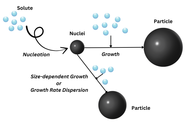
Fig. 8 Nucleation, growth and growth rate dispersion in PBM. Note that dispersion is used to model (random) variance in growth speed, not the reduction of particle size.

Population Balance Model in a CSTR

We assume a well-mixed tank and choose the particle size \(x\in (x_c, \infty)\) as the internal coodinate, with \(x_c>0\) being the minimal particle size considered. The corresponding PBM is given as

\[\begin{aligned} \frac{\partial (n V)}{\partial t} = F_{in}n_{in} - F_{out}n - V \left( \frac{\partial (v_{G}n)}{\partial x} - D_g \frac{\partial^2 n}{\partial x^2} - B_0 \delta (x-x_c) \right), \end{aligned}\]

where \(F_{in}, F_{out}\in \mathbb{R}^+\) are the volumetric inflow and outflow rates, \(V\in\mathbb{R}^+\) is the reactor volume, \(n(t, x)\colon [0, T_\text{end}] \times (x_c, \infty) \mapsto \mathbb{R}^+\) is the number density distribution, \(n_{in}\in\mathbb{R}^+\) is the number density distribution of the inlet feed, \(v_{G}\in\mathbb{R}^+\) is the particle growth rate, \(D_g\in\mathbb{R}^+\) is the growth dispersion rate.

The boundary conditions are given by the regularity boundary condition

(28)\[\begin{aligned} \left. \left( nv_{G} - D_g \frac{\partial n}{\partial x} \right) \right|_{x \to \infty}=0, \end{aligned}\]

and the nucleation kinetics boundary condition

(29)\[\begin{aligned} \left. \left( nv_{G}-D_g \frac{\partial n}{\partial x} \right)\right|_{x=x_c} = B_0, \end{aligned}\]

where \(B_0\in\mathbb{R}^+\) is the nucleation kinetics factor representing particle nucleations of size \(x_c\in\mathbb{R}^+\).

The model is complemented by the following mass balance equation which accounts for the mass transfer between the particle phase and the solute phase

\[\begin{aligned} \frac{\partial (cV)}{\partial t} = F_{in}c_{in} - F_{out}c -\rho k_v V \left( B_0x^3_c + 3\int_{x_c}^{\infty} v_{G}n\ x^2 \;\mathrm{d}x \right), \end{aligned}\]

where \(c(t)\colon [0, T_\text{end}] \mapsto \mathbb{R}^+\) is the solute concentration in the bulk phase, \(c_{in}\in\mathbb{R}^+\) is the inlet solute mass concentration, \(\rho > 0\) is the nuclei mass density and \(k_v > 0\) is the volumetric shape factor of the particles.

Evolution of the reactor’s volume is governed by

\[\begin{aligned} \frac{\mathrm{d}V}{\mathrm{d}t} &= F_{\text{in}} - F_{\text{out}}. \end{aligned}\]

Population Balance Model in a DPFR

The PBM can also be formulated for a DPFR to model continuous processes. That is, we choose the axial position within a DPFR as the external coordinate \(z\in[0, L]\) and formulate the \(2D\) PBM

\[\begin{aligned} \frac{\partial n}{\partial t} = -v_\text{ax} \frac{\partial n}{\partial z} +D_{ax} \frac{\partial^2 n}{\partial z^2} - \frac{\partial (v_{G}n)}{\partial x} + D_g \frac{\partial^2 n}{\partial x^2}, \end{aligned}\]

where \(n(t, x, z)\colon [0, T_\text{end}] \times (x_c, \infty) \times [0, L] \mapsto \mathbb{R}^+\) is the number density distribution, \(v_\text{ax}\in\mathbb{R}^+\) is the axial velocity and \(D_{ax}\in\mathbb{R}^+\) is the axial dispersion coefficient.

Boundary conditions for the internal coordinate are again given by Eq. 28 and Eq. 29.

For the external coordinate \(z\), Danckwerts boundary conditions are applied:

\[\begin{aligned} \left. \left( n v_\text{ax}-D_{ax}\frac{\partial n}{\partial z} \right) \right|_{z=0} = v_\text{ax} n_{in,x}, \qquad \left.\frac{\partial n}{\partial z}\right|_{z=L}=0. \end{aligned}\]

The mass balance equation for the solute \(c(t, z)\colon [0,T-\text{end}] \times [0,L] \mapsto \mathbb{R}^+\) is given by

\[\begin{aligned} \frac{\partial c}{\partial t} = -v_\text{ax} \frac{\partial c}{\partial z} +D_{ax} \frac{\partial^2 c}{\partial z^2} -\rho k_v \left( B_0x^3_c + 3\int_{x_c}^{\infty} v_{G}n x^2 \;\mathrm{d}x \right). \end{aligned}\]

As for the particle phase, the solute mass concentration subjects to the Danckwerts boundary conditions

\[\begin{aligned} \left.\left( c v_\text{ax}-D_{ax}\frac{\partial c}{\partial z} \right) \right|_{z=0} = v_\text{ax} c_{in}, \qquad \left.\frac{\partial c}{\partial z}\right|_{z=L}=0. \end{aligned}\]

Constitutive equations

Constitutive equations describe the kinetic processes in the governing equations. The relative supersaturation \(s>0\) is:

\[\begin{aligned} s=\frac{c-c_{eq}}{c_{eq}}, \end{aligned}\]

where \(c_{eq}>0\) is the solute solubility in the solvent. The nucleation kinetics can be split into primary and secondary nucleation:

\[\begin{aligned} B_0 = B_p + B_s, \end{aligned}\]

Which are in turn defined by the following constitutive equations. An empirical equation for primary nucleation is given by:

\[\begin{aligned} B_p=k_ps^u, \end{aligned}\]

where \(k_p\in\mathbb{R}^+\) is the primary nucleation rate constant and \(u\in\mathbb{R}^+\) is a constant. An empirical power-law expression is used for the secondary nucleation:

\[\begin{aligned} B_s=k_bs^bM^k, \end{aligned}\]

where \(k_b\in\mathbb{R}^+\) is the secondary nucleation rate constant, \(b\in\mathbb{R}^+\) and \(k\in\mathbb{R}^+\) (usually set to \(1\)) are system-related parameters and \(M\in\mathbb{R}^+\) is the suspension density defined as

\[\begin{aligned} M=k_v\rho\int_{0}^{\infty}n\ x^3\;\mathrm{d}x. \end{aligned}\]

The following expression for the growth rate is implemented:

\[\begin{aligned} v_{G}=k_gs^g(a+\gamma x^p), \end{aligned}\]

where \(k_g\in\mathbb{R}^+\) is the growth rate constant, \(\gamma\in\mathbb{R}^+\) quantifies the size dependence, and \(g, a, p\in\mathbb{R}^+\) are system-related constants.

For information on model parameters and how to specify the model interface, see Crystallization / Precipitation models.